Transfer learning is popular in image recognition tasks due to its ability to leverage the knowledge learned from a pre-trained model to improve the performance of a new model.
Transfer learning is a machine learning technique that allows a model trained on one task to be applied to a different but related task. This allows the model to improve its performance on a new task without requiring it to be trained from scratch. Transfer learning is particularly useful in cases where there is a limited amount of data available. It is commonly used in fields such as natural language processing and image recognition.
Many transfer learning algorithms have been developed in image recognition. Examples of networks used in those algorithms include:
- VGGNet: This is a convolutional neural network (CNN) developed by the Visual Geometry Group at the University of Oxford.
- ResNet: Another CNN model developed by Microsoft Research that has been widely used as a pre-trained model for image recognition tasks. It is known for its ability to train without suffering from the problem of vanishing gradients.
- Inception: This is a CNN developed by Google that has been used as a pre-trained model for tasks such as object detection and image classification. It is known for its efficient use of computational resources and good performance on various image recognition tasks.
- AlexNet: This is a CNN developed by Alex Krizhevsky, Ilya Sutskever, and Geoffrey Hinton that was one of the first deep learning models to achieve state-of-the-art performance on the ImageNet dataset.
- MobileNet: This is a CNN developed by Google that is designed to be lightweight and efficient, making it well-suited for use on mobile devices.
In this article, we are going to create an image recognition model using transfer learning to classify images based on logos they contain. Transfer learning will be used to fine-tune a pre-trained model on a dataset of logos to improve its ability to detect and classify them on new images.
You can run this code on Google Colab.
First, you will need to obtain a dataset of logos that you want to detect. This dataset will include a set of images with different logos of brands. You can create this dataset yourself by manually collecting and labeling images, or you can use one of the existing datasets. In this example, we will be using the Flickr Logo 27 dataset.
The Flickr Logo 27 dataset is a dataset of 27 classes of brand logos that were collected from the Flickr website.
!pip install wget
_URL = 'http://image.ntua.gr/iva/datasets/flickr_logos/flickr_logos_27_dataset.tar.gz'
wget.download(_URL)
We need to extract the zip files.
import tarfile

file1 = './flickr_logos_27_dataset.tar.gz'

if file1.endswith("tar.gz"):
    tar = tarfile.open(file1, "r:gz")
    tar.extractall()
    tar.close()

file2 = './flickr_logos_27_dataset/flickr_logos_27_dataset_images.tar.gz'

if file2.endswith("tar.gz"):
    tar = tarfile.open(file2, "r:gz")
    tar.extractall()
    tar.close()
Now, we need to create lists of labels and images from the CSV annotation file:
import pandas as pd
from keras.utils import np_utils
from sklearn.model_selection import train_test_split
from keras.preprocessing import image
from PIL import ImageFile
from sklearn.preprocessing import LabelEncoder

data = pd.read_csv("./flickr_logos_27_dataset/flickr_logos_27_dataset_training_set_annotation.txt", sep='\s+',header=None,index_col=None)

variables= data.iloc[:, [0,1]]
encoder = LabelEncoder()
variables['Nlabel'] = encoder.fit_transform(variables.iloc[:, [1]])
variables.drop(variables.columns[1], axis=1,inplace=True)
url= '/content/flickr_logos_27_dataset_images'
list_label = [ ]
list_Image = [ ]
list_file_actual = [ ]
print(variables)
for Image, Label in variables.values:
list_label.append( Label)
img = tf.keras.utils.load_img(url+'/'+Image, target_size=(128, 128))
x = tf.keras.utils.img_to_array(img)
x = np.expand_dims(x, axis=0)
list_Image.append(x)
list_label = np.array(list_label)We need to split the total dataset into training and validation datasets and save them as tensors needed for training.
train_files, val_files, train_targets, val_targets = train_test_split(list_Image, list_label, test_size=0.2, random_state=42)
train_files=np.vstack(train_files)
val_files= np.vstack(val_files)
train_tensors = train_files.astype('float32')/255
val_tensors = val_files.astype('float32')/255
Next, you will need to select a pre-trained model to use for transfer learning. For this example, we will use the Mobilenet model, which is a popular choice for object detection and recognition tasks. We will load the base model without the top layers and then create the head layers that are specific for this transfer learning task and attach them on top of the base model.
For the base model, we will load the MobileNetV2 model without the top:
baseModel = MobileNetV2(weights="imagenet", include_top=False,input_shape=train_tensors.shape[1:])Then, we will define anAveragePooling2D layer that performs average pooling on the output of the base model. Pooling is typically used to downsample the spatial dimensions of a tensor, such as reducing the height and width of a tensor by a factor of 2 or more. This can help reduce the number of parameters in the model and reduce overfitting, which is a common problem with deep learning models, as well as reduce the computational cost of training the model.
headModel = baseModel.output
headModel = AveragePooling2D(pool_size=(4, 4))(headModel)
Then, we are going to define a Flattenlayer that flattens the output of the pooling layer. It is typically used to reshape a multi-dimensional tensor into a single vector, for example, a 10×10 matrix into a 100×1 vector. This is often necessary before passing the output through a dense layer, which expects a one-dimensional input, that is, a vector.
headModel = Flatten(name="flatten")(headModel)
headModel = Dense(128, activation="relu")(headModel)
Then, we will set a dropout layer. The Dropout layer is a regularization technique for reducing overfitting in neural networks. It works by randomly setting a fraction of the values in the input tensor to 0 during training, which helps prevent the model from relying too heavily on any feature.
Lastly, we will set a Dense layer with 27 classes (recall we are working with the Flickr 27 logo dataset). The output of this layer is typically a vector of probabilities, where each element in the vector represents the probability of the input belonging to a particular logo class. The class with the highest probability is chosen as the final prediction of the model.
headModel = Dropout(0.5)(headModel)
headModel = Dense(27, activation="softmax")(headModel)

model = Model(inputs=baseModel.input, outputs=headModel)

for layer in baseModel.layers:
 layer.trainable = False

# compile our model
model.compile(loss="sparse_categorical_crossentropy", optimizer='Adam',metrics=["accuracy"])
You can run this command to see the architecture of our model:
model.summary()We will set the following variables, which are also known as hyperparameters of the model: the height and width of the pixelated image data, the number of training epochs, and the batch size of data per epoch.
HEIGHT = 128
WIDTH = 128
EPOCHS =  100
Let’s train our model:
H = model.fit(train_tensors, train_targets, epochs=EPOCHS, verbose=1,
                  validation_data=(val_tensors, val_targets))
Let’s plot the training and validation accuracy and loss curves. We expect the loss values to decrease with the number of epochs and the accuracy values to increase with the number of epochs.
# plot the training loss and accuracy
N = EPOCHS
plt.style.use("ggplot")
plt.figure()
plt.plot(np.arange(0, N), H.history["loss"], label="train_loss")
plt.plot(np.arange(0, N), H.history["val_loss"], label="val_loss")
plt.title("Training Loss VS Validation Loss")
plt.xlabel("Epoch #")
plt.ylabel("Loss/Accuracy")
plt.legend(loc="lower left")
plt.show()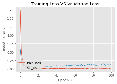
N = EPOCHS
plt.style.use("ggplot")
plt.figure()
plt.plot(np.arange(0, N), H.history["accuracy"], label="train_acc")
plt.plot(np.arange(0, N), H.history["val_accuracy"], label="val_acc")
plt.title(" Accuracy")
plt.xlabel("Epoch #")
plt.ylabel("Accuracy")
plt.legend(loc="lower left")
plt.show()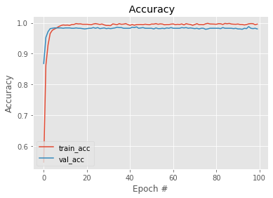
We will define the ‘predict image’ function to classify any new image by passing the path to the image as an argument.
from PIL import Image
def predimage(path):
    fig = plt.figure(figsize =(5, 4))
    image = Image.open(path)
    plt.imshow(image)
    test = load_img(path,target_size=(WIDTH,HEIGHT))
    test = img_to_array(test)
    test = np.expand_dims(test,axis=0)
    test /= 255
    result = model.predict(test)
    im_class = np.argmax(result[0], axis=-1)
    print(encoder.inverse_transform([im_class]))
Let’s test the model on a new image:
predimage('/content/sprite.webp')This is the result:
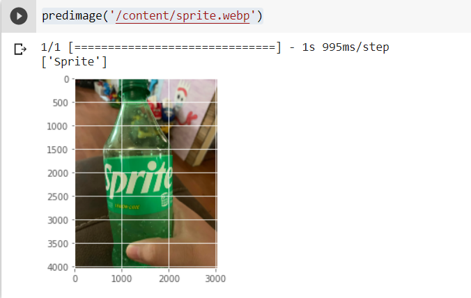
It’s important to note that the accuracy of the model will depend on the quality and diversity of the dataset used to train the classifier. To improve the performance of the model, you may want to consider using a larger and more diverse dataset to fine-tune the pre-trained model. Other parts of the algorithm, e.g., the hyperparameters, can also be tweaked to improve the prediction accuracy
Here is the code on Google Collab: https://colab.research.google.com/drive/1FvFzdqPEQXRLWAW98ITM9b9w98i_WEyz?usp=sharing
Resources:
- Xception! – Flickr27 : Brand Logo Detection
- Classifying Logos in Images with Convolutionary Neural Networks (CNNs) in Keras
Image Recognition with Transfer Learning: A Case Study in Logo Classification was originally published in Eydle on Medium, where people are continuing the conversation by highlighting and responding to this story.